Mie Scattering of Gold Nanospheres: Lumerical FDTD and COMSOL vs. Mie Theory
Published:
Updated October 10, 2026.
After I chose plasmonic nanoparticles as my research field back in 2015, the first thing my advisor asked me to do was to reproduce the Mie scattering of gold nanoparticles using Lumerical FDTD, a numerical solver developed by Lumerical Inc., which was acquired by Ansys in 2020, the year I graduated. It was the first time I realized the power of modeling or simulation. Since then I have enjoyed comparing things, e.g., comparing theory with experiment, comparing different theories or methods. I have now used Lumerical FDTD (sorry Ansys, I still prefer to call it Lumerical FDTD) for more than seven years. I have also been modeling nanophotonics problems with COMSOL Multiphysics, another popular numerical solver, for a long time, yet I still think it is a great exercise to look at this problem, namely, Mie scattering of plasmonic nanoparticles, the phenomenon that makes plasmonic nanoparticles colorful and interesting in nanophotonics and photocatalysis. In this tutorial, I will walk you through the modeling process and we will compare our modeling result with the analytical solution, Mie theory.
Mie Theory
Mie theory is an exact analytical solution to Maxwell’s equations for spheres of arbitrary size and thus can be used to calculate the optical spectra, which essentially is an electromagnetic problem, of spherical particles, given that the dielectric functions of the particle and the environment are known. Rather than go through the development and derivation of Mie theory, which I believe deserves another tutorial, let’s take its solution for granted for now and keep in mind that it is an analytical approach.
The general expressions for the scattering and extinction cross-sections from Mie theory are
\[\sigma_\mathrm{sca}=\frac{2\pi R^2}{x^2}\sum_{n=1}^\infty(2n+1)(|a_n|^2+|b_n|^2),\] \[\sigma_\mathrm{ext}=\frac{2\pi R^2}{x^2}\sum_{n=1}^\infty(2n+1)\mathrm{Re}[a_n+b_n],\]where $x=2\pi Rn_\mathrm{m}/\lambda$, $n_\mathrm{m}$ is the refractive index of the medium, $R$ is the radius of the particle, and the absorption cross-section is given by $\sigma_\mathrm{abs}=\sigma_\mathrm{ext}-\sigma_\mathrm{sca}$. The $a_n$ and $b_n$ factors are given by
\[a_n=\frac{\psi'_n(mx)\psi_n(x)-m\psi_n(mx)\psi_n'(x)}{\psi'_n(mx)\zeta_n(x)-m\psi_n(mx)\zeta'_n(x)},\] \[b_n=\frac{m\psi'_n(mx)\psi_n(x)-\psi_n(mx)\psi'_n(x)}{m\psi'_n(mx)\zeta_n(x)-\psi_n(mx)\zeta'_n(x)},\]where $\psi_n(z)=(\pi z/2)^{1/2}\times J_{n+1/2}(z)$, $\zeta_n(z)=(\pi z/2)^{1/2}\times(J_{n+1/2}(z)+iY_{n+1/2}(z))$ and $m=n_\mathrm{p}/n_\mathrm{m}$, where $n_\mathrm{p}$ is the refractive index of the particle (written as $n+ik$, the sign convention that goes with the Hankel function of the first kind). The different terms in eqs. 1 and 2 correspond to the dipole ($n=1$), quadrupole ($n=2$), and so on. Don’t be intimidated if the expressions for $\psi_n$ and $\zeta_n$ look complicated and unfamiliar; they are just special functions (spherical Bessel and Hankel functions of the first kind) and they are usually built-in functions in scientific computing languages, e.g. MATLAB.
You may wonder: what if the nanoparticle is not a sphere? What if the shape is complicated enough that finding an analytical solution is impractical? Well, thanks to the development of applied mathematics, we now have a general solution: the numerical approach. In fact, the numerical methods, such as the finite-difference time-domain (FDTD) method, finite element method (FEM), and discrete dipole approximation (DDA), for electromagnetic problems have led to a subject called computational electromagnetics. In the following sections, we will use Lumerical FDTD, which, as the name suggests, is a solver based on the FDTD method, and COMSOL Multiphysics, which is an FEM solver, to model the scattering phenomenon from gold nanoparticles. Since we also have the exact analytical solution, it doesn’t hurt to compare the numerical results with it. So, let’s go!
Finite-Difference Time-Domain Method Simulation in Lumerical FDTD
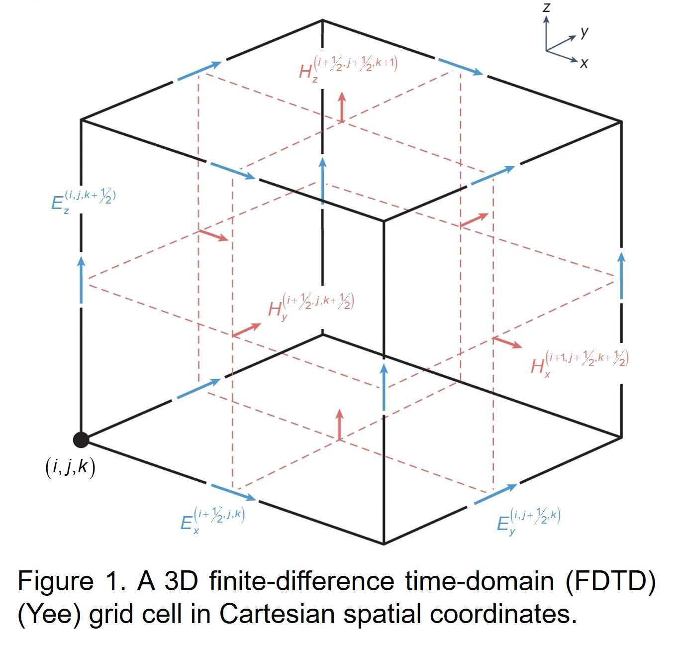
The finite-difference time-domain (FDTD) method is a direct space method, first introduced by Yee in 1966. It solves the time-domain form of Faraday’s law and the Ampère–Maxwell law (eqs. 5 and 6) to obtain the time evolution of electric and magnetic fields across a spatial grid (Yee grid cell).
\[\mu\frac{\partial\mathbf{H}}{\partial t}=-\nabla\times\mathbf{E}-\mathbf{M},\] \[\varepsilon\frac{\partial\mathbf{E}}{\partial t}=\nabla\times\mathbf{H}-\mathbf{J_s}-\sigma_\mathrm{c}\mathbf{E},\]in which $\mathbf{E}$ is the electric field, $\mathbf{H}$ is the magnetic field, $\mathbf{J_s}$ is the electric current density source and $\mathbf{M}$ is the equivalent magnetic current density. Also, note that we have three primary constitutive parameters of materials to describe the electromagnetic properties:
\[\mathbf{D}=\varepsilon\mathbf{E},\] \[\mathbf{B}=\mu\mathbf{H},\] \[\mathbf{J}=\sigma_\mathrm{c}\mathbf{E},\]in which $\varepsilon$ is the electric permittivity, $\mu$ is the magnetic permeability and $\sigma_\mathrm{c}$ represents the conductivity.
Materials and objects of interest are generally placed into the Yee grids (Figure 1) and assigned constitutive material parameters based on the cell location. Central differencing is then used to approximate the time and spatial partial derivatives in eqs. 5 and 6. Truncating the Taylor series expansions of the field components yields a second-order accurate scheme in both space and time. The resulting time-domain fields can then be converted into the frequency or wavelength domain through the Fourier transform.
Since we are interested in the absorption and scattering of electromagnetic waves by spherical nanoparticles, we need to introduce a source in our simulation. There are numerous source options for an FDTD model: hard, soft, resistive voltage, and plane wave sources. In our case, we select plane waves as our source, and in particular, we will model the plane waves from a distant source using the total-field scattered-field formulation.
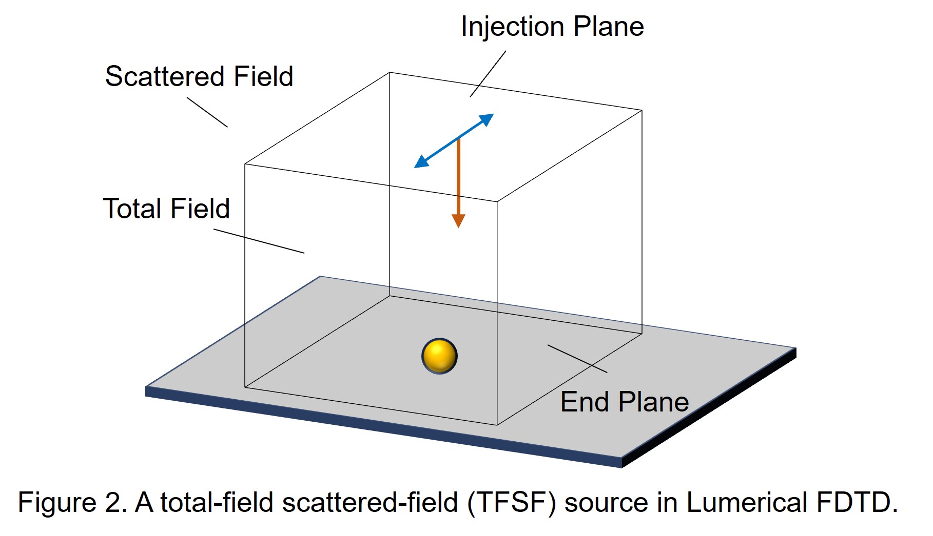
\[\mathbf{E}=\mathbf{E}_\mathrm{total}=\mathbf{E}_\mathrm{background}+\mathbf{E}_\mathrm{scattered}.\]It turns out that this special plane wave source is a built-in source in Lumerical FDTD: the TFSF source (Figure 2).
In addition to the objects (materials), grids, and sources, we need appropriate boundary conditions in any numerical simulation. For instance, perfect electric conductor (PEC) and perfect magnetic conductor (PMC) reflect electromagnetic waves and can be very useful to take advantage of certain types of symmetries in simulation. Periodic boundary conditions (PBCs), such as Bloch boundary conditions, are useful when modeling periodic structures, e.g., metasurfaces. And absorbing or radiation boundary conditions are suitable for open-region problems to avoid infinite simulation regions and to minimize spurious reflections along the outer boundaries of the grid. Among many absorbing boundary conditions, the perfectly matched layer (PML) is the most popular one because of its overall efficiency and robustness, and we will use it in our Mie scattering simulation. And guess what, the PML boundary conditions are the default boundary conditions once we add an FDTD region in Lumerical FDTD.
It should be noted that usually one or several dependent variables are solved for in any numerical solver; for instance, we solve for $\mathbf{E}$ and $\mathbf{H}$ in Lumerical FDTD. It is then our job to connect the dependent variables to the quantities we want: the cross-sections in Mie scattering. Since the cross-sections are defined as the ratio of power (either absorbed or scattered, unit: $\mathrm{W}$) to input power density (unit: $\mathrm{W/m^2}$), and the input power density is a parameter we can control in the simulation, we just need to know the absorbed or scattered power. We can make the connection between dependent variables $\mathbf{E}$ and $\mathbf{H}$ to power through Poynting vectors:
\[P=\int\int(\mathbf{n}\cdot\mathbf{S})dA,\]where $P$ is power, $\mathbf{n}$ is the normal vector of the surface under study, $\mathbf{S}=\frac{1}{2}\mathrm{Re}(\mathbf{E}\times\mathbf{H}^*)$ is the time-averaged Poynting vector, and $dA$ is the surface element. Let’s assume the input power density is $I_0$, then the cross-sections are calculated as:
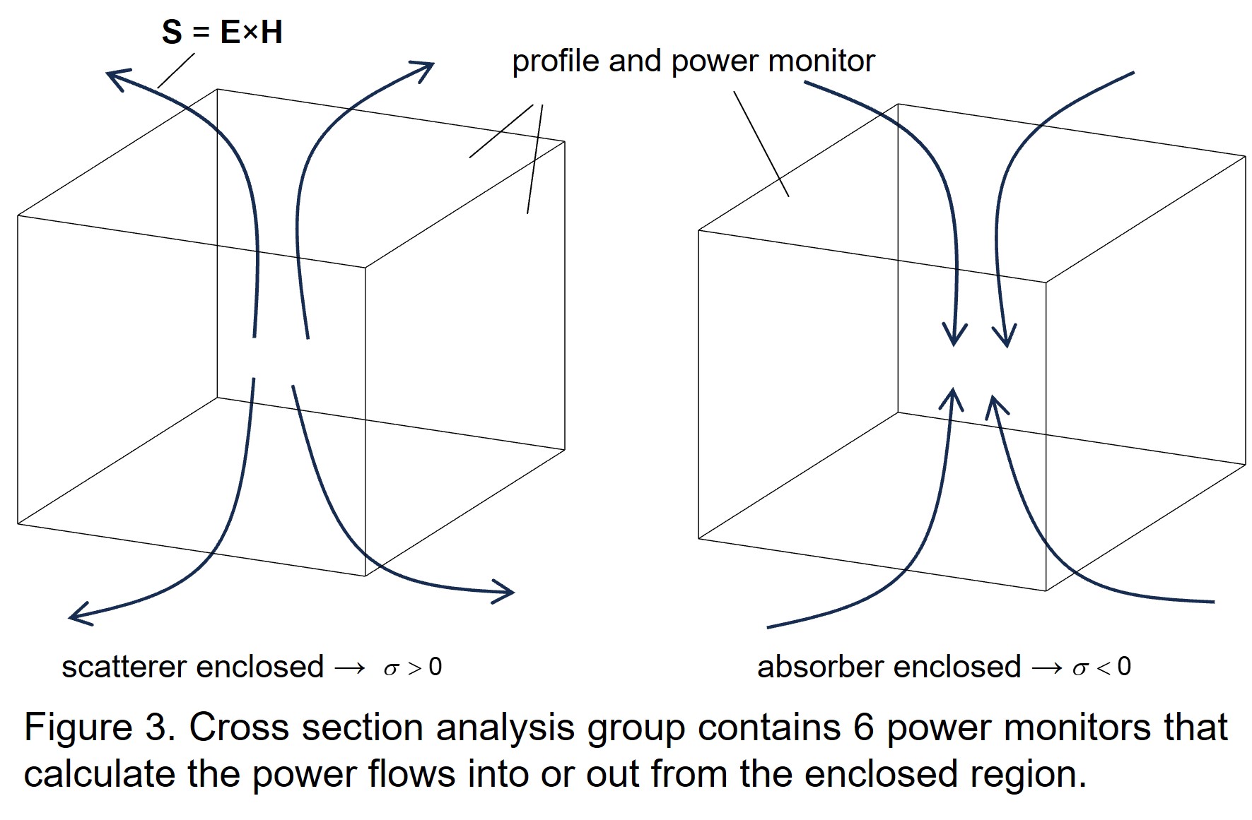
\[\sigma=\frac{P}{I_0}=\frac{1}{I_0}\int\int(\mathbf{n}\cdot\mathbf{S})dA.\]Seems complicated? Don’t worry, it turns out that Lumerical FDTD has many built-in functions and even analysis groups to help us out. For instance, the transmission script command can be applied to a power monitor (an object we can place in Lumerical FDTD) to get the amount of power transmitted through it. And the built-in Cross section analysis group consists of six power monitors enclosing a region and analyzing the net power flowing into or out of that enclosed region (Figure 3). Note that for absorption the output cross-section is a negative quantity but it is just due to the convention used in Lumerical FDTD. So we just need to put one Cross section analysis group inside the TFSF source to capture the absorption cross-section, and put another outside the TFSF source, where only the scattered field is present (Figure 2), to calculate the scattering cross-section.
Therefore, the procedure for setting up a Lumerical FDTD simulation of Mie scattering is:
- Set up the simulation region (Simulation $\rightarrow$ Add FDTD region), and note that the outer boundary of the simulation region defaults to PML. So make sure the simulation region is large enough so the evanescent tails of the resonant surface plasmon modes will not interact with the PML boundary conditions.
- Put a gold nanosphere at the center of the simulation (Structures $\rightarrow$ Sphere) and edit its radius as you want. Make sure to change the material to Au.
- Put a TFSF source (Sources $\rightarrow$ Total-field scattered-field) enclosing the gold nanosphere. Set the wavelength from 400 nm to 700 nm; this range is suitable to capture the localized surface plasmon resonance of gold nanospheres.
- Insert a Cross section analysis group (from Analysis $\rightarrow$ Optical power $\rightarrow$ Cross section) inside the TFSF source, and edit its dimensions to enclose the gold nanosphere. This analysis group will calculate the absorption cross-section.
- Insert another Cross section analysis group to enclose the TFSF source. This analysis group will calculate the scattering cross-section.
- For higher accuracy, override the mesh setting by inserting a user-defined mesh (Simulation $\rightarrow$ Mesh).
- Optionally, modify the wavelength or frequency data points in Monitors $\rightarrow$ Global properties to get a nice-looking spectrum.
By following the steps above, we should be able to get the simulation files looking like these, in which I have set up and finished the simulation for gold nanospheres with radii of 30 nm and 80 nm. And the result can be viewed by right-clicking the Cross section analysis groups (Run analysis, and then Visualize). There is one more thing that I haven’t told you yet about the optical constants I used in the simulation; I will touch on that after we discuss COMSOL Multiphysics.
Finite Element Method Simulation in COMSOL Multiphysics
The finite element method (FEM) is another numerical method that is used to solve boundary-value problems characterized by a partial differential equation and a set of boundary conditions. It is a more general method than the finite-difference time-domain method, and thus can also be applied to other physics governed by other partial differential equations, such as heat transfer, stress analysis, mass diffusion, etc. In FEM, the geometrical domain of the boundary-value problem, for instance, the gold nanosphere and its surroundings in our case, is discretized using sub-domain elements, called the finite elements, and the differential equation is applied to a single element after it is brought to the weak form. Then a set of shape functions (also known as interpolation functions) is used to represent the primary unknown variable, e.g., the electric field $\mathbf{E}$, in the element domain. A set of linear equations is obtained for each element in the discretized domain. Finally, a global matrix system is formed after the assembly of all elements.
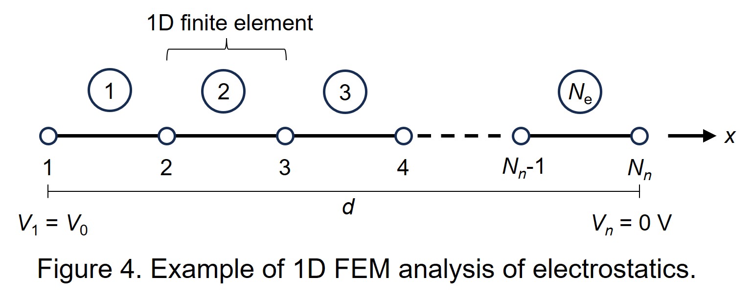
Before we dive into the modeling process in COMSOL Multiphysics, let’s look at a one-dimensional problem of electrostatics (Figure 4) to get a better understanding of FEM. As shown in Figure 4, we are curious about the spatial profile of electric potential $V$ between two parallel conducting plates separated by a distance $d$. We divide the geometry into $N_e$ elements (segments), which gives $N_n=N_e+1$ nodes. The left plate (node 1) is maintained at a fixed potential $V_1 =V_0$, while the right plate (the last node, labeled $V_n$ in Figure 4) is grounded, $V_n = 0\;\mathrm{V}$. To complete the physical picture, let’s say the medium between the two plates is nonmagnetic with a dielectric constant $\varepsilon_r$ and a uniform electron volume charge density $\rho_v=-\rho_0$ is also present in the medium.
The (partial) differential equation associated with the above problem is Poisson’s equation:
\[\nabla\cdot(\varepsilon_r\nabla V)=-\frac{\rho_v}{\varepsilon_0}.\]Since the medium between the two plates is homogeneous, linear, and isotropic, the above equation can be converted into
\[\frac{d^2V}{dx^2}=\frac{\rho_0}{\varepsilon_r\varepsilon_0}.\]In FEM, briefly, we need to find the values of the solution at the nodes that make the weighted residual of the governing partial differential equation vanish, and then one may use linear interpolation to find approximate solutions between two nodes. Two common approaches for finding solutions at nodes are the variational approach and the method of weighted residuals. Instead of going through every detail of FEM, let’s use the method of weighted residuals as an example to demonstrate what the weak form is in the FEM.
The solution inside the $e^{th}$ element can be written as
\[V=\sum_{j=1}^qv_j^eN_j(x),\]where $v_j^e$ are the solution values at the nodes of the element, $N_j(x)$ are the governing interpolation functions (e.g., polynomial of degree one), and $q$ is the number of nodes in the domain of the element; since we are considering a 1-D linear element, $q=2$.
The weighted residual is formed by moving all terms of the differential equation above to one side, multiplying by a weight function $w(x)$, and integrating over the domain of the element. The resulting weighted residual for a single element has the following form:
\[r^e=\int_{x_1^e}^{x_2^e}w[\frac{d}{dx}(\varepsilon^e\frac{dV}{dx})+\rho_v]dx,\]where $x_1^e$ and $x_2^e$ are positions of the left and right nodes of the element, and $\varepsilon^e=\varepsilon_r^e\varepsilon_0$ is the permittivity of the medium inside the element.
We then seek an approximate solution for $V$ by forcing the weighted residual to be zero and thus obtain a weighted-integral equation
\[\int_{x_1^e}^{x_2^e}w[\frac{d}{dx}(\varepsilon^e\frac{dV}{dx})+\rho_v]dx=0.\]The above equation is the weighted-residual form of the governing differential equation; the differential equation itself (eq. 14) is the strong form.
For each (arbitrary) choice of weight function $w(x)$, an equation is formed with unknowns being the values of the electrostatic potential at the nodes of the element. It is often preferred that the weight functions $w(x)$ be identical to the interpolation or shape functions $N(x)$. This approach is known as the Galerkin finite element method.
It is evident that the interpolation functions $N(x)$ must be twice differentiable. This stringent requirement can be relaxed by using integration by parts to trade the double differentiation of $V(x)$ for a single differentiation of each of $V(x)$ and $w(x)$:
\[\int_{x_1^e}^{x_2^e}w\frac{d}{dx}(\varepsilon^e\frac{dV}{dx})dx=\int_{x_1^e}^{x_2^e}wd(\varepsilon^e\frac{dV}{dx})=w\varepsilon^e\frac{dV}{dx}\bigg|_{x_1^e}^{x_2^e}-\int_{x_1^e}^{x_2^e}(\frac{dw}{dx})\varepsilon^e(\frac{dV}{dx})dx.\]Then, the weak form is:
\[\int_{x_1^e}^{x_2^e}(\frac{dw}{dx})\varepsilon^e(\frac{dV}{dx})dx-\int_{x_1^e}^{x_2^e}w\rho_vdx-w\varepsilon^e\frac{dV}{dx} \bigg|_{x_1^e}^{x_2^e}=0.\]One can prove that the weak and strong forms are equivalent. Thanks to the weak form, we can use linear algebra with matrices and vectors to represent the partial differential equation in that finite element, and the assembly of all finite elements leads to a global matrix equation. Once the global matrix equation is solved, we can obtain the electric potential $V$ at each node and the regions in between two nodes are interpolated using interpolation functions $N_j(x)$ from every node.
Even the one-dimensional case above is complicated enough that software such as MATLAB is typically used to reach the desired accuracy. You can imagine that for a three-dimensional problem, it would be almost impractical to do FEM by hand, and this is where COMSOL Multiphysics comes in.
COMSOL Multiphysics is a popular FEM solver and it is backed by hundreds of engineers and scientists who wrote fast and reliable algorithms so we can perform the electromagnetic simulation using FEM in a reasonable time. COMSOL Multiphysics is also accompanied by various modules and the one we are using here is the Wave Optics Module. However, COMSOL Multiphysics is just an FEM solver; it is our job to define parameters, create objects, define material properties, and set up boundary conditions to perform simulation.
The procedures of setting up a simulation in COMSOL Multiphysics are very similar to those in Lumerical FDTD: define simulation region, create objects, define material properties, introduce source, and set up appropriate boundary conditions. However, two things differ: 1) COMSOL Multiphysics allows two formulations, Full field and Scattered field, in Electromagnetic Waves, Frequency Domain (ewfd), one of the physics interfaces of the Wave Optics Module. By choosing Scattered field, we restrict ourselves to only the scattered field (eq. 10) and we need to provide the expression of the background field; 2) the scattering power is calculated similarly as in eq. 11. Because we choose the Scattered field formulation, however, the absorbed power is calculated using a built-in expression of total power dissipation density ewfd.Qh = ewfd.Qml + ewfd.Qrh, where ewfd.Qml is the magnetic losses and ewfd.Qrh is the resistive losses.
The absorbed power is the volume integral of their sum, $P_\mathrm{abs}=\int\int\int\mathrm{ewfd.Qh}dV$, performed for the gold nanosphere only.
Here are the simulation files in COMSOL Multiphysics that solved the Mie scattering of gold nanospheres with radii of 30 nm and 80 nm.
Comparison
Figure 5 summarizes the results from analytical solutions (solid lines), solutions from COMSOL Multiphysics (filled circles), and solutions from Lumerical FDTD (empty squares). As expected, both numerical results match well with the analytical solution. In terms of physics, we see that the absorption process dominates in small nanospheres while the scattering process is much more prominent for larger nanoparticles. This suggests that people should use small nanoparticles to harness plasmonic hot carriers, an intermediate stage during the absorption process.
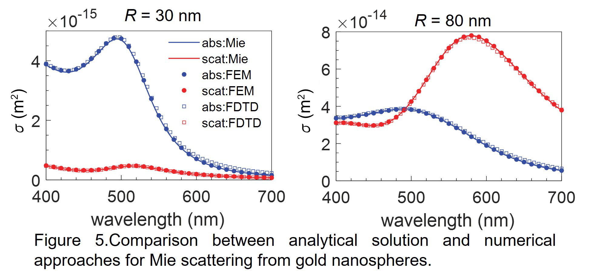
Remember the one thing I hadn’t told you: the optical constants I used in Lumerical FDTD. To get a better comparison, I exported the optical constants of gold that I used in COMSOL Multiphysics and imported them into Lumerical FDTD and the Mie calculation. Otherwise, the tiny difference in optical constants used in different approaches might result in slight discrepancies in the end.