Updated October 10, 2026.

In the previous tutorial, I mentioned that the nonradiative damping of surface plasmons was historically viewed as a loss in the field of nanophotonics;¹ however, it is now a popular topic in the community of photocatalysis and photochemistry: chemists have realized that the “losses”, if managed properly, can be turned into advantages to drive (uphill) chemical reactions and can even demonstrate certain bond selectivity that is not accessible by thermal means.

The advantages are associated with energetic nonthermal or hot carriers that are generated after nonradiative damping of surface plasmons; it would therefore be useful if one could predict the energy distribution of nonthermal carriers for a given plasmonic nanoparticle. Indeed, there are multiple ways to perform such calculations, ranging from free-electron models^{2, 3} to more rigorous treatments based on density functional theory (DFT).^{4, 5}

During my Ph.D. study and postdoctoral work, I followed ref. 2 to calculate the energy profile of nonthermal carriers and then applied it to model the tunneling current⁶ and photocatalytic performance.⁷ It turns out that the approach used here could also serve as an extracurricular activity for first-year graduate students or senior undergraduates to strengthen their understanding of quantum chemistry. In fact, the main result of ref. 2 can be reproduced by simply combining quantum chemistry and entry-level electromagnetics. Let’s get started!

Preliminary Knowledge

Fermi’s Golden Rule

“In quantum physics, Fermi’s golden rule is a formula that describes the transition rate (the probability of a transition per unit time) from one energy eigenstate of a quantum system to a group of energy eigenstates in a continuum, as a result of a weak perturbation” — Wikipedia.

Fermi’s golden rule is the tool that we will use to analyze our problem, since we are interested in the transition probability of exciting an electron (hole), after nonradiative decay of excited plasmons, from its initial state to all possible final states. Therefore, before I throw you into a math puzzle, let me walk you through the fundamentals of Fermi’s golden rule. (You can also find the derivation of Fermi’s golden rule in many textbooks and online materials.)

The modeling of plasmonic nonthermal carriers is essentially a perturbation problem. For now, let’s assume the perturbation is a constant value $H’$ (we will consider the effect of localized surface plasmon later); the Hamiltonian of the system can be written as

where $H_0$ is the unperturbed Hamiltonian and $H’$ represents the perturbation. Let’s say the unperturbed wavefunction $\Psi_0$ satisfies the time-dependent Schrödinger equation (TDSE):

where the wavefunction $\Psi_0$ has the generic form:

Since the Hamiltonian (Energy) operator is a Hermitian operator, its eigenfunctions shall form a complete set. Let’s use $\vert u\rangle$ to represent the eigenfunctions of $H_0$, that is, $\vert u\rangle=\lbrace u_1^0,u_2^0,\dots,u_n^0\rbrace$. Because any wavefunction can be represented as a linear combination of the eigenfunctions (if these eigenfunctions form a complete set), eq. 3 can be written more generally as

The subscript and superscript $0$ denote the unperturbed system. The unperturbed state described by $H_0$ has a set of energy eigenvalues such that

By comparing eq. 3 and eq. 4 at $t=0$, it is easy (hopefully for you as well) to tell that $\psi_0(\mathbf{r})=\sum_na_n^0u_n^0$ (a wavefunction can be described as a linear combination of a complete orthonormal set $\vert u\rangle$). Note that the expansion coefficients $a_n^0$ are independent of time.

Suppose now we have a state described by wavefunction $\Psi$, and we are interested in how this wavefunction evolves (after the perturbation $H’$). We then put the wavefunction $\Psi$ in eq. 1 and use the TDSE

and

Note that now the prefactors $a_n(t)$ depend on time. Substituting eq. 7 into eq. 6, multiplying by the complex conjugate $u_s^{0*}$ and using the orthonormality of the wavefunctions, we obtain

where

The $\int\mathrm{d}\tau$ denotes integration over the full range of all the coordinates of a system.

For a small perturbation, the time variation of $a_n(t)$ is slow, so $a_n(t)\cong a_n(0)$ and

where

For simplicity, consider the special case in which the system is in state $n$ at $t=0$, that is, $a_n(0)=1$ and all other $a_{s\neq n}(0)=0$. Then

Eq. 12 shows that $H’(t)$ can induce transitions from state $n$ to other states ($s\neq n$).

If $H’$ is independent of time,

Therefore,

Now we can perform some mathematical tricks on eq. 14,

Since $\lim\limits_{x\rightarrow 0}\mathrm{sinc}(x)=1$, for short times eq. 15 becomes

Thus, the short-time behavior is quadratic in time.

In the long-time limit ($t\rightarrow\infty$), we also rewrite eq. 14 as

Here, we’ve defined $\Delta E=E_s-E_n=\omega_{sn}\hbar$. Let us further define a function $D_t(\Delta E)\equiv4\sin^2(\frac{\Delta Et}{2\hbar})/(\Delta E)^2$ and plot $D_t(\Delta E)$ vs. $\Delta E$ to visualize its properties (Figure 1).

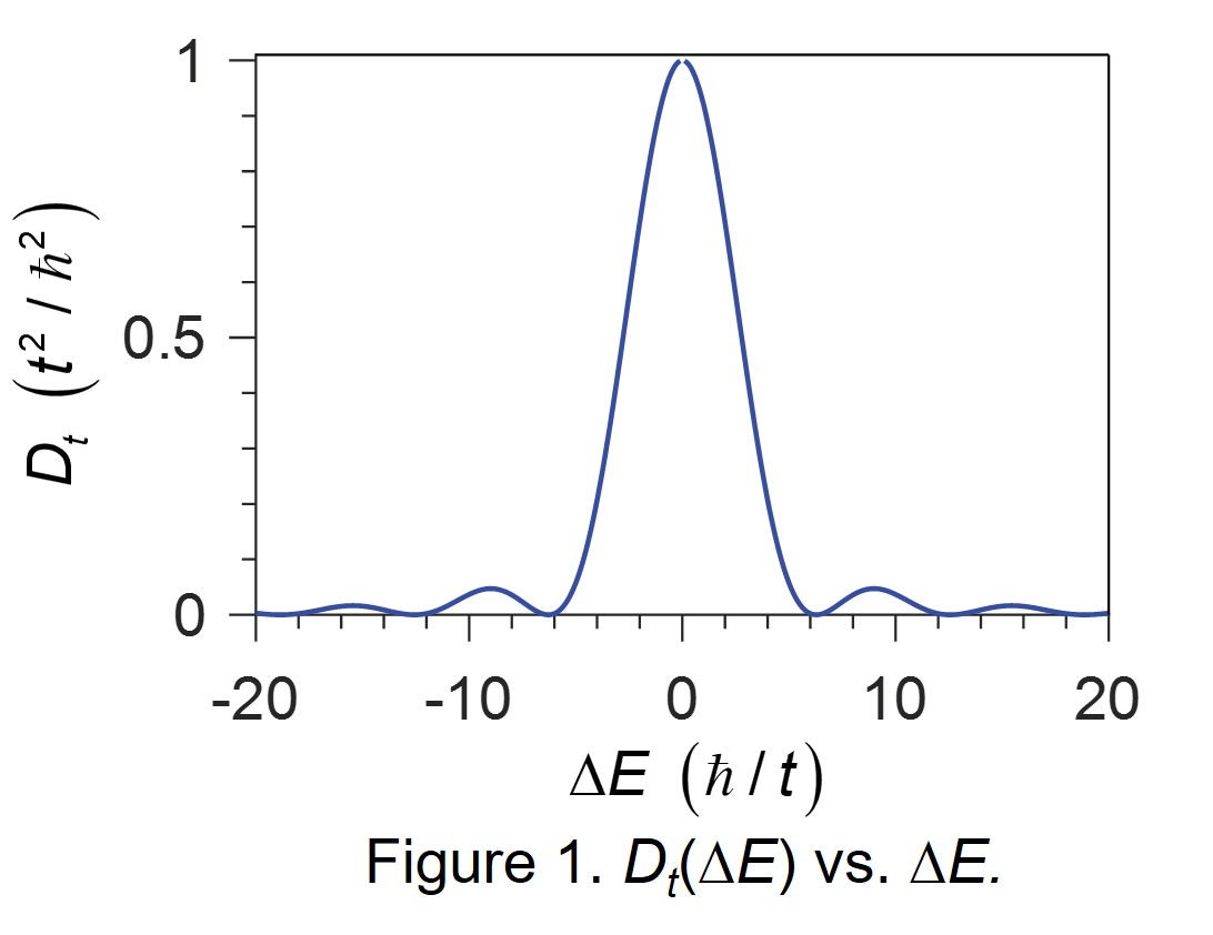
Figure 1 shows that $D_t(\Delta E)$ has large values only for $-2\pi\hbar/t<\Delta E<2\pi\hbar/t$, where the maximum $D_t(0)=t^2/\hbar^2$ increases rapidly with time. Furthermore, since $\int_{-\infty}^\infty D_t(x)\mathrm{d}x=2\pi t/\hbar$, we define another function

which is a representation of the $\delta$-function in the limit $t\rightarrow\infty$.

If we plug eq. 18 into eq. 17,

And the transition rate $R=\mathrm{d}P/\mathrm{d}t$ becomes

Eq. 20 is indeed the well-known Fermi’s golden rule.

Harmonic Perturbation

So far, we’ve only considered the constant perturbation, that is, $H’$ is independent of time once it is turned on. Now we consider the interaction with an oscillating perturbation turned on at time $t_0=0$ (Figure 2). The results will be used to describe how a light field induces transitions in a system through dipole interactions.

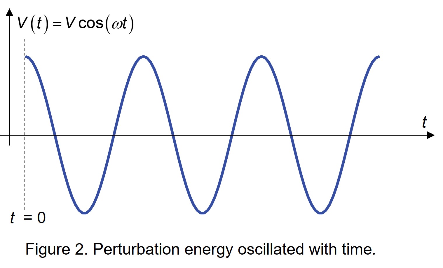
Again, we want to know the rate of transition between states $n$ and $s$. Here, we treat the light field classically:

Setting $t_0\rightarrow 0$ and substituting eq. 22 into eq. 12,

Since $e^{i\theta}-1=2ie^{i\theta/2}\sin(\theta/2)$, eq. 23 becomes

The first term in eq. 24 is absorption, and the second is stimulated emission.

Notice that the terms in eq. 24 are only significant when $\omega\approx\pm\omega_{sn}$, that is, a matching of the frequency of the harmonic interaction with the transition energy between quantum states (Figure 3).

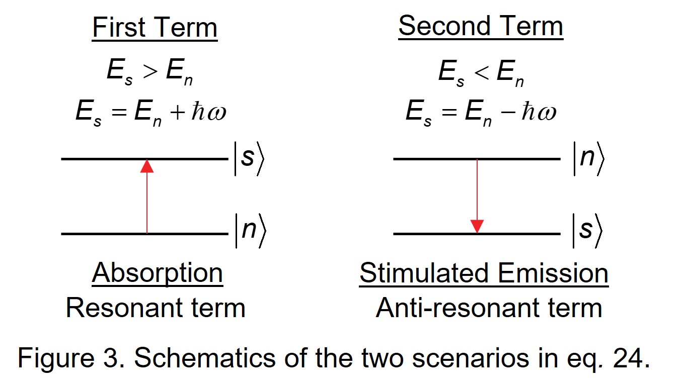
We first analyze the absorption part:

We then do a similar transformation as in eqs. 17–18,

Note that $\Delta E$ here is defined as $\Delta E\equiv\hbar(\omega_s-\omega_n-\omega)$. The transition rate for this absorption process is therefore

Similarly, the transition rate for the stimulated emission process is

The overall transition rate (probability per unit time) from state $n$ to state $s$ is then

Note that in the long-time limit, we neglect interference between the resonant and anti-resonant terms.

Furthermore, the Dirac delta function can be expressed as a Lorentzian to account for the relaxation process,

Note here that we define $\hbar\omega_s\equiv\varepsilon_f$ and $\hbar\omega_n\equiv\varepsilon_i$; the subscripts $f$ and $i$ denote the final and initial states.

By introducing a damping factor $\gamma=\hbar/\tau$ in eq. 30, and substituting eq. 30 in eq. 29 (note that we switched notation here: $M_{fi}=V_{sn}/2$ is the matrix element of the $e^{-i\omega t}$ component of the perturbation in eq. 22, so $\vert M_{fi}\vert^2=\vert V_{sn}\vert^2/4$), we obtain

After accounting for the spin and the occupation probability dictated by the Fermi–Dirac distribution, eq. 31 becomes

If one considers all the possible initial states, eq. 32 becomes eq. 1 of ref. 2.

Wavefunctions of Spherical Nanoparticles

Then we need to find the appropriate basis set for conduction electrons in plasmonic nanoparticles. For simplicity, we consider nanoparticles with a spherical shape, which leaves us with a central-force problem when solving the Schrödinger equation:

where $\nabla^2\equiv\frac{\partial^2}{\partial x^2}+\frac{\partial^2}{\partial y^2}+\frac{\partial^2}{\partial z^2}$.

For a sphere, it is convenient to work in spherical coordinates, so we rewrite the Laplace operator in spherical coordinates,

It can be shown that (in any quantum mechanics/chemistry book)

where $\hat{L}$ is the angular momentum operator.

Therefore, eq. 33 is transformed to

And it can also be shown that

Thus, it is possible to have a set of simultaneous eigenfunctions of $\hat{H}$, $\hat{L}^2$, and $\hat{L}_z$ for the central-force problem,

Using the above eigenvalues, eq. 36 can be transformed as

The eigenfunctions of $\hat{L}^2$ are spherical harmonics $Y_l^m(\theta, \phi)$, and since $\hat{L}^2$ does not involve $r$, it is possible to multiply $Y_l^m$ by an arbitrary function of $r$ and still have eigenfunctions of $\hat{L}^2$ and $\hat{L}_z$.

Plugging the variable-separated wavefunction into eq. 39 and dividing both sides by $Y_l^m$, one gets an ordinary differential equation for the unknown function $R(r)$

Then we transform eq. 41 a little bit and then look up the mathematical solution (sometimes a friend majoring in mathematics is a plus),

Try $R$ as $y(x)$ and $x=kr$, $k=\sqrt{\frac{-2m(V(r)-E)}{\hbar^2}}$. This substitution is only valid where $V(r)$ is constant, so that $k$ does not depend on $r$; for the spherical potential well considered below, that is the case inside and outside the sphere separately.

Thus, eq. 42 becomes

Since $x=\sqrt{\frac{-2m(V(r)-E)}{\hbar^2}}r$, the above equation becomes

It turns out that eq. 45 has analytical solutions: the two linearly independent solutions are spherical Bessel functions of the first kind $j_l$ and spherical Bessel functions of the second kind $y_l$.

Finite Spherical Potential Well

Instead of an infinite potential well, as quantum chemistry textbooks usually consider, here we consider a more realistic scenario (Figure 4), that is, the potential inside the spherical nanoparticles, of radius $r_0$ (labeled $R$ in Figure 4), has a finite value $V_0$, and the potential outside the nanoparticle is $0$ (vacuum level).

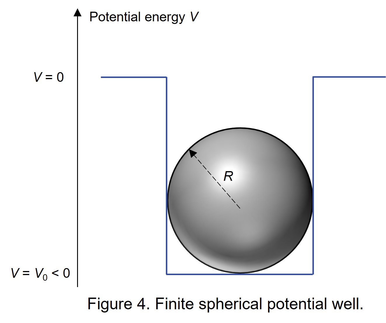
Note that $V_0$ is negative here, and the bound states we are looking for have energies $V_0<E<0$. From eq. 46, one may write down the wavefunction inside the nanosphere, which is $\psi_\mathrm{in}=j_l(kr)$ with $k=\sqrt{\frac{2m(E-V_0)}{\hbar^2}}$. Outside the sphere the potential is $0$ and $E<0$, so the wavefunction must decay with distance: $\psi_\mathrm{out}=k_l(\kappa r)$ with $\kappa=\sqrt{\frac{-2mE}{\hbar^2}}$, where $k_l(x)$ is the modified spherical Bessel function of the second kind. It is purely real, and it is equivalent (up to a constant factor) to the spherical Hankel function of the first kind, $h_l(x)=j_l(x)+iy_l(x)$, evaluated at the imaginary argument $i\kappa r$.

Then we need to apply boundary conditions to find eigenenergies: the wavefunction needs to be continuous and smooth. Continuity requires that the wavefunctions match at the surface of the nanosphere, while smoothness requires that their first derivatives also match at the surface.

Rather than solving the two conditions separately, the logarithmic derivative is used instead

which reads

Then the allowed energy (implicitly included in $k$ and $\kappa$) can be found by searching for the roots of eq. 49. We can repeat this procedure for all possible $l$, and Figure 5a summarizes these results for a $D=25\;\mathrm{nm}$ silver sphere. Furthermore, we can also visualize the broadened density of states (DOS), as shown in Figure 5b; it matches well with the three-dimensional free-electron-gas models in solid-state physics as expected.

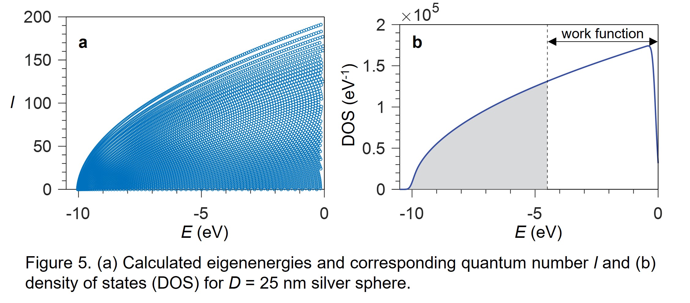
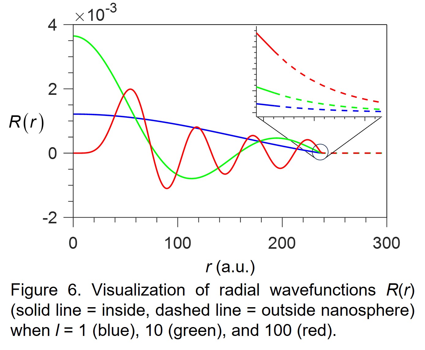
The parameter $V_0$ is crucial since it determines the material’s work function. For the $D=25\;\mathrm{nm}$ Ag nanosphere in Figures 5 and 6, we choose $V_0=-10.04\;\mathrm{eV}$ to ensure the correct work function ($\sim4.5\;\mathrm{eV}$). For a wavefunction to be well-behaved, we require it to be normalized, $\int_{-\infty}^\infty \psi^*\psi\mathrm{d}\tau=1$. After normalization, we can pick three random state wavefunctions of the same $D=25\;\mathrm{nm}$ sphere (Figure 6) to visualize that the boundary conditions are fulfilled. As shown in Figure 6, the wavefunctions we found are indeed continuous and smooth across the interface (solid line for inside the sphere, and dashed line for outside the sphere).

Nonthermal Carrier Generation

Now we have all the tools we need to calculate the generation rate and energy distribution of nonthermal carriers: we are equipped with the formula derived from Fermi’s golden rule and the wavefunctions to describe the conduction band electrons in nanospheres. By looking at eq. 32, we realize the only remaining puzzle is the transition matrix element $M_{fi}=\langle\psi_f\vert eV’\vert\psi_i\rangle$, where $V’$ is the overall potential that electrons feel when the illumination is on. The overall potential for nanospheres can be written as $V’=V_{ext}+V_p$, where $V_{ext}$ is the external potential and $V_p$ is the plasmon-induced potential; the latter can be written as (from entry-level electromagnetics books):

And the external perturbation is simply $V_{ext}=-E_0r\cos\theta$. For silver, we use the Drude model $\varepsilon=\varepsilon_\mathrm{b}-\frac{\omega_{pl}^2}{\omega^2+i\omega\gamma_p}$ with background dielectric function $\varepsilon_\mathrm{b}=4.18$, a plasma frequency $\omega_{pl}=9.07\;\mathrm{eV}$, and a plasmon damping of $\gamma_p=60\;\mathrm{meV}$.²

One more trick to note: the transition matrix element is evaluated as

where $v(r)$ is the radial part of the overall potential, defined through $V’=E_0v(r)\cos\theta$. Luckily, we do not need to deal with the explicit expression: it turns out that $\vert\langle Y_{l_f}^{m_f}\vert\cos\theta\vert Y_{l_i}^{m_i}\rangle\vert^2$ can be evaluated analytically as

where $l_\mathrm{min}$ is the smaller of $l_f$ and $l_i$. Note the selection rule is that $l_f-l_i=\pm 1$ and $m_f=m_i$.

Finally, we can put everything together and evaluate the transition probability per unit time (equivalently, the excitation rate) using eq. 32, this time for a $D=15\;\mathrm{nm}$ silver nanosphere (Figure 7). For comparison, we also show the results from ref. 2 alongside.

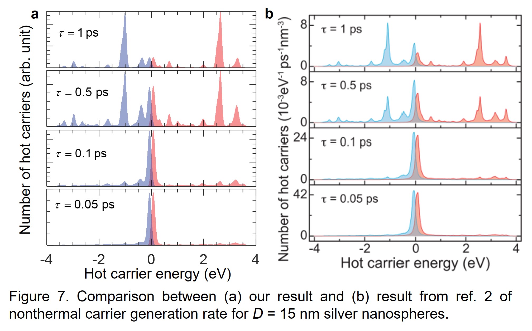
Note: the axes of Figure 7 are labeled “hot carriers”, following the terminology of ref. 2. The carriers calculated here are the nonthermal carriers in the sense of the previous tutorial: they are generated directly by plasmon decay and have not yet relaxed into a Fermi–Dirac-like distribution. Much of the literature uses the two terms interchangeably.

If you are interested in the detailed MATLAB code to perform this calculation, please email me at joeysxwu@gmail.com.

References

1. Khurgin, J. B. How to deal with the loss in plasmonics and metamaterials. Nat. Nanotechnol. 10, 2–6 (2015).
2. Manjavacas, A., Liu, J. G., Kulkarni, V. & Nordlander, P. Plasmon-induced hot carriers in metallic nanoparticles. ACS Nano 8, 7630–7638 (2014).
3. Govorov, A. O., Zhang, H. & Gun’ko, Y. K. Theory of photoinjection of hot plasmonic carriers from metal nanostructures into semiconductors and surface molecules. J. Phys. Chem. C 117, 16616–16631 (2013).
4. Sundararaman, R., Narang, P., Jermyn, A. S., Goddard, W. A. III & Atwater, H. A. Theoretical predictions for hot-carrier generation from surface plasmon decay. Nat. Commun. 5, 5788 (2014).
5. Brown, A. M., Sundararaman, R., Narang, P., Goddard, W. A. III & Atwater, H. A. Nonradiative plasmon decay and hot carrier dynamics: effects of phonons, surfaces, and geometry. ACS Nano 10, 957–966 (2016).
6. Wu, S. & Sheldon, M. T. Optical power conversion via tunneling of plasmonic hot carriers. ACS Photonics 5, 2516–2523 (2018).
7. Wu, S., Chen, Y. & Gao, S. Plasmonic photocatalysis with nonthermalized hot carriers. Phys. Rev. Lett. 129, 086801 (2022).